Industrial chiller sizing in the plastics industry: how to calculate the required cooling capacity

Q_cooling = Q_melt + Q_hydraulics + Q_other

Three terms. Most requests for quotation leave out two of them, and then wonder why the chiller cannot cope in summer.

There is a widely circulated rule of thumb for sizing cooling capacity: a quarter of a kilowatt for every kilogram of plastic processed per hour. It is quick, easy to remember, and in practice it regularly misses by a wide margin. This article walks through the proper calculation on a single, concrete machine, then scales it up to a six-machine plant.

The worked example is built on injection moulding, but the underlying methodology carries over to other industries: breaking the heat sources down into items, separating the temperature levels, checking the water side separately, and selecting the machine for the actual operating point. The specific items and the parts concerning mould geometry, however, are plastics-industry specific.

Why is this worth the effort? Because cooling is by far the longest phase of the injection moulding cycle (our article on the basics of industrial cooling covers the technologies in detail): with thermoplastics it can account for as much as two-thirds of the total cycle time. Whatever is a bottleneck in cooling shows up directly in the part cost.

And the rule of thumb is not enough because it tries to condense several mutually independent heat sources into a single number, and their proportions differ completely from plant to plant. The type of material processed can change half of it. So can the machine's drive technology. Let us take them in order.

01. Melt heat: the material matters a lot

The first item is the heat that has to be extracted from the molten material so that the part can be ejected. The formula is simple:

Q_melt [kW] = throughput [kg/h] × Δh [kJ/kg] ÷ 3600

Δh is the specific enthalpy difference between the melt temperature and the ejection temperature. And here is the point most tables keep quiet about: with semi-crystalline materials (PP, PE, PA, POM) Δh also includes the latent heat of crystallisation. This heat leaves while the temperature does not drop at all. That is why the polypropylene in our example needs nearly twice as much cooling as the same amount of polystyrene.

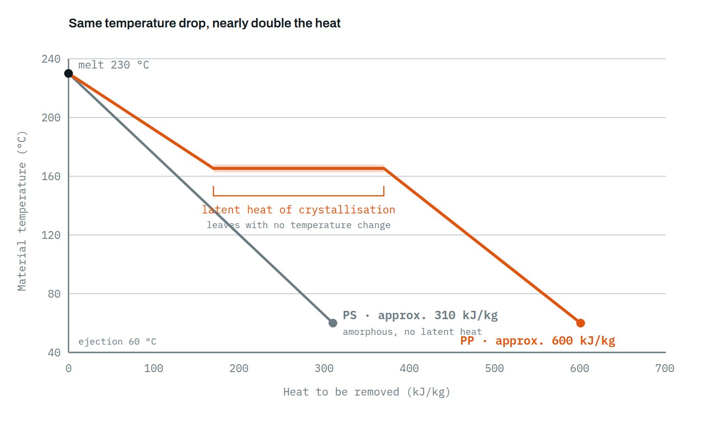
Indicative design values (230 → 60 °C)

Material	Structure	Δh (kJ/kg)	kW / (kg/h)
PS / ABS	amorphous	300–320	0.085
PC	amorphous	300	0.083
PET	semi-crystalline	400	0.110
PP	semi-crystalline	600	0.167
PA 6	semi-crystalline	600	0.167
PE-HD	semi-crystalline	650–700	0.190

These are indicative design values, not material constants. The actual Δh depends on the specific grade, the degree of crystallinity, and the assumed start and end temperatures. Wherever available, always use the material supplier's datasheet.

Let us take a concrete machine: a 150-tonne hydraulic injection moulding machine, PP material, 15 kg/h throughput.

15 × 600 ÷ 3600 = 2.5 kW

Why enthalpy rather than the classic specific-heat formula?

Many plants and several training materials use the old, simpler formula:

Q = material quantity × specific heat × temperature difference

It is important to state that the two methods can only be compared directly for identical start and end states. Our table refers to 230 °C down to 60 °C; if someone calculates with a different melt or end temperature, the two results are not describing the same thing in the first place.

The specific-heat formula has a substantive limitation regardless: it does not explicitly handle the latent heat of crystallisation or the temperature dependence of specific heat. It treats plastic like steel or water, assuming that specific heat is constant and there is no phase change. With a semi-crystalline material there is one: the heat of crystallisation leaves without any drop in temperature, and the specific heat is not the same in the melt and in the solid state either.

With amorphous materials (PS, ABS, PC) there is no latent heat of crystallisation, so the specific-heat approximation generally causes a smaller error there. With PP, PE, PA and POM, however, the latent heat is a substantial item, and in those cases the enthalpy method is more reliable. This is one of the reasons why a chiller that looks sufficient on paper still cannot cope in practice.

There is a circumstance that masked the difference for a long time: the old formula is often applied down to the mould temperature, even though the part is ejected warmer than that. This overly large temperature difference biases the result upwards and partly offsets the missing latent heat. But the two errors are not equal in size and do not always point in the same direction, so their cancellation must not be relied on.

Running total · 150 t hydraulic machine · PP · 15 kg/h

Melt heat	2.5 kW
So far	2.5 kW

The mould and its surroundings: which way does the heat flow?

It is a fair question whether this 2.5 kW is not too little for a mould. The number is correct, but it is worth knowing what it means: this is the energy that has to be extracted from the polymer. How much of it ends up in the cooling water depends on what the mould does with its surroundings.

And the direction of the heat is not self-evident here. The temperature of the mould's outer surfaces is neither that of the water nor that of the cavity, but somewhere between the two. If this surface is warmer than the hall air, the mould gives off heat and less load lands on the water. If it is colder, the opposite happens: the hall and the clamping platens heat the mould, and the water has to carry that away too.

Which case applies? Roughly speaking, this decides it:

• Warm mould (materials requiring higher mould temperatures, hot runner, high specific throughput): the outer surface is well above hall temperature, the mould loses heat, which reduces the water-side load. Its magnitude depends on the mould's surface area, its surface temperature, the hall temperature and the air movement, so it can only be calculated case by case.
• Cold mould (low water temperature, low specific throughput): the outer surface may drop below hall temperature. In that case the environment and the massive clamping platens feed heat into the mould, which is an additional load. At low specific throughput this case is more likely, because little melt heat arrives, but kg/h alone does not decide it.

In the opposite direction, one item always adds: the radiation of the plasticising unit and the contact of the nozzle carry heat into the mould. With a hot-runner mould, the loss of the heated manifold ends up in the mould plates, and the cooling water has to remove that as well. The latter is not negligible, and it must be calculated separately, using the hot-runner manufacturer's data.

The practical conclusion: the 2.5 kW is the machine-side base load of the cold loop, based on the polymer. The items of the specific mould's heat balance must be added to or subtracted from it, and this has to be done mould by mould.

The dew point is the hidden limit if there is no mould-space drying

A cold mould has a more serious consequence than dry heat gain. If the mould surface drops below the dew point of the hall air, moisture condenses on it. That means rust and surface defects on the part, and the condensation also adds a further, potentially significant latent heat load.

Concretely: in a 25 °C hall at 50 percent relative humidity the dew point is around 14 °C; at 60 percent it is already 17 °C, and at 70 percent it is above 19 °C. A 15 °C mould loop can therefore easily drop below the dew point in summer, in a humid hall.

So the question in sizing is not how cold you can go, but how cold you are allowed to. If the central chilled-water network runs at 7 °C, for example, the mould loop can be operated at a higher temperature by mixing or with a temperature control unit. The cold water then remains a reserve, not an automatic operating setpoint.

There is an exception: mould-space drying systems exist that prevent condensation and thereby allow mould temperatures below the dew point. Where such a system is installed, the limit lies elsewhere.

02. Hydraulic oil: this is where drive technology really counts

A significant part of the electrical power drawn by the pump does not go into the part but turns into heat in the oil: across throttles, valves and internal leakage. On a classic, fixed-speed hydraulic machine the oil-cooling load is a considerable share of the power drawn.

In our worked example we use a multiplier of 0.65. It is important to clarify that this is an example assumption, not a design standard. If manufacturer heat-load data or your own measurement is available, always use that instead.

It also matters how old a machine we are calculating with. Our example is a 15–20-year-old, classic, fixed-speed hydraulic machine.

It is worth knowing that several differing estimation methods are in circulation for this item. Some start from the installed drive-motor power with a fixed fraction, some from the cycle-average power drawn, and the industry sizing guides do not use the same ratio either. Our 7.2 kW is one possible estimate, not an industry truth. If you have manufacturer heat-load data or a measurement, it overrides all of them.

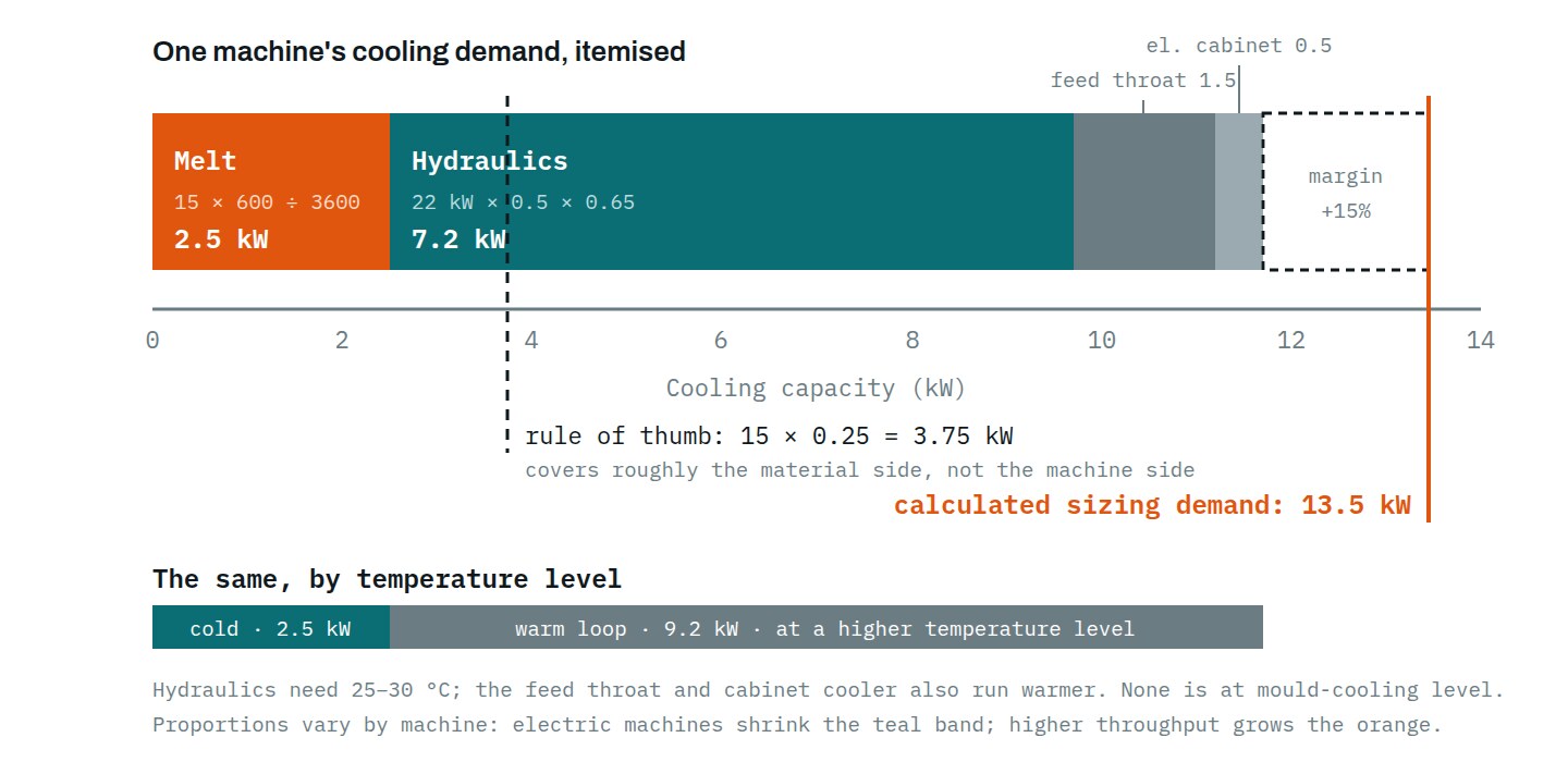
Our machine's installed drive motor is 22 kW; the real cycle average is roughly half of that, so 11 kW. With the assumption above, about 7.2 kW of this lands in the cooling water.

The cycle average is itself an assumption, and strongly cycle-dependent. In production with longer cooling times and lower specific throughput it is typically lower. This too is worth taking from measurement if you have the means.

Importantly, the hydraulic heat load does not scale with kg/h but with the cycle and the drive technology. With servo-hydraulics this is particularly visible: in the cooling and idle phases the controlled pump motor can even stop, which meaningfully reduces the oil heat load.

This is the highest-variance point of the sizing. On newer machines this item is markedly smaller, and on servo-hydraulic machines it is significantly smaller. For hybrid and servo-hydraulic drives, machine manufacturers specifically highlight the reduction in cooling-water and oil demand compared with conventional hydraulics, in some cases communicating a demand smaller by roughly a third. On an all-electric machine the machine's own cooling-water demand drops further, although the exact extent depends on machine size and configuration. So if your machine park is younger, do not carry this item over from the example under any circumstances.

The practical consequence: in a plant that has switched to electric machines, the old chiller easily becomes oversized. And an oversized chiller works with short compressor cycles and poor part-load efficiency. This is not a theoretical risk but one of the most common reasons why a well-run plant has a high specific energy cost for cooling.

Running total · 150 t hydraulic machine · PP · 15 kg/h

Melt heat	2.5 kW
Hydraulic oil (22 kW × 0.5 × 0.65)	7.2 kW
So far	9.7 kW

03. The "other" that is not negligible

• Feed throat temperature control: 1–2 kW per machine. It looks small, but with ten machines it is already a complete smaller chiller.
• Electrical cabinet cooling: 0.5–1 kW per machine if a water-cooled cabinet cooler is installed. This item is almost always left out of the sizing, even though it runs continuously — even while the machine is standing still.
• On blow moulding machines, separately: blow-pin cooling. It cools the neck of the formed bottle directly, so it genuinely requires cold water, and it directly affects the cycle time as well.
• Dryers, compressors, granulators: if they are connected to the same loop, they must be included.

What not to count twice

Do not count again the process heat that the temperature control unit removes from the mould. That heat is already included in the melt heat; if you enter it a second time, you pay for the same kilowatt twice.

This does not mean the TCU is thermally neutral. Its own pump loss, its heating and its other incidental heat loads may enter the system — these must be assessed separately. Only the process heat must not be double-counted.

The feed throat is a special case

It is worth being precise here, because the terms are easy to mix up. For sizing purposes it is not the material hopper that matters but the temperature control of the feed throat, i.e. the water cooling around the machine's intake zone (called the feed throat in machine manufacturers' documentation). Machine manufacturers treat these two separately.

The feed throat temperature must be controlled depending on machine and material: heat migrates continuously upwards from the barrel, while overcooling is also a problem for material arriving from the dryer. The required water temperature and the actual heat load must be determined from the machine manufacturer's data, not from a general empirical value.

What we can pin down for sizing: this is not the temperature level of mould cooling. The feed throat's heat load therefore does not automatically belong on the chiller. For our example machine, based on the manufacturer's data: 1.5 kW feed throat and 0.5 kW electrical cabinet.

Running total · 150 t hydraulic machine · PP · 15 kg/h

Melt heat	2.5 kW
Hydraulic oil	7.2 kW
Feed throat	1.5 kW
Electrical cabinet	0.5 kW
Cooling demand per machine	11.7 kW

A concept that will accompany the calculation from here on

The four items do not occur at the same temperature level, and at the end of the sizing this will be of decisive importance. Mould cooling genuinely asks for cold water, typically between 7 and 15 °C. The hydraulic oil is fine with 25–30 °C, the feed throat runs warmer still, and the electrical cabinet cooler is practically satisfied with ambient level.

It is therefore worth splitting the items into two groups now; the rest of the article will refer to them by these names:

• Cold loop: what genuinely requires a chiller. In our example machine this is the 2.5 kW of mould cooling.
• Warm loop: what can be removed at a higher temperature level. The remaining 9.2 kW: hydraulics, feed throat and cabinet cooling.

What size and type of equipment this turns into is calculated in section 8. Until then it is enough that only the smaller part of the heat load is what a compressor is needed for.

04. From one machine to a plant: coincidence and margin

So far we have looked at a single machine. Let us scale it up to a typical mid-sized plant.

The example plant: six broadly identical, 150–200-tonne hydraulic injection moulding machines, all processing PP. The raw total is 6 × 11.7 = 70.2 kW.

What the 15 kg/h means — this matters

The 15 kg/h per machine is the average throughput during production, not an average over the shift. If your figure already includes downtime, do not reduce again in the step below, because that would average twice.

What not to reduce by

A common argument is that the machines do not inject at the same moment, so the total can be reduced. From the heat-load point of view this does not hold. The chiller does not see shot-by-shot peak power but a heat load smoothed over time: the heat capacity of the water in the system absorbs the cycle-by-cycle fluctuation. It does not matter that one machine injects three seconds later.

Moreover, our calculation already works with averages. The 15 kg/h is an average throughput, and the 11 kW is a cycle average. Putting a further reduction factor on top, citing cycle offsets, would average the same thing twice.

The productive-hours ratio alone is not enough

Here lies the quiet error of most sizing exercises. It seems obvious to argue that, according to production control, say 80 percent of machine hours are productive hours, so multiply by 0.80.

For an energy average calculation that is a fine figure. For chiller capacity sizing it is not enough. The chiller does not have to handle the shift average but the sustained simultaneous load. Six machines can average 80 percent productive while all six run simultaneously for several hours a day. Those few hours size the equipment, not the average.

You may therefore only reduce if you have time-series data showing how many machines load the system simultaneously and continuously. That is no longer a productive-hours ratio but a coincidence factor, and the two are not the same. If you only have the former, do not reduce.

And even with such data, not equally on every item

If you do have time-series coincidence data, you still must not apply it to the whole total in one go.

Melt heat is directly proportional to production: if the machine does not inject, there is no melt. The hydraulic load largely follows production too, though not linearly.

The feed throat temperature control, however, keeps running while the machine stands but the barrel stays hot — including during mould changes and start-up. And the electrical cabinet cooling operates as long as the machine is under voltage. Do not scale these down unless they genuinely stop together with the machine.

Margin: overprovisioning is also a design error

A chiller sized at double works in short compressor cycles, wears faster, runs at worse part-load efficiency, and needlessly ties up the investment budget. In the example we use a 15 percent margin.

Importantly, this 15 percent specifically covers the uncertainty of the machine-side estimates: the material data, the hydraulics estimate, the feed throat and cabinet cooling values. It does not cover the loop's own loads (pump, piping, condensation), because those are not yet known at this point. At final equipment selection the reserve must therefore be re-evaluated, now with the full heat balance in hand.

Our example plant has no time-series coincidence data, only a productive-hours ratio. Therefore we do not reduce.

Machine-side base load · 6-machine plant · PP

Melt heat · 6 × 2.5	15.0 kW
Hydraulics · 6 × 7.2	43.2 kW
Feed throat · 6 × 1.5	9.0 kW
Electrical cabinet · 6 × 0.5	3.0 kW
Subtotal × 1.15 margin	80.7 kW
If a 0.80 coincidence figure existed for the production-dependent items	67.3 kW
Machine-side base load	80.7 kW

What this means in practice

Without data: 80.7 kW. This is the correct starting point if all you know is that the machines do not run continuously. The faint 67.3 kW row would only be valid if time-series load data proved that the production-dependent items load the system at no more than an 80 percent level even on a sustained basis.

There is 13 kW between the two, which in this size range is roughly a full machine-size step. In other words, it pays to request the hourly load time series from production control before asking for quotations.

What you should not do: do not guess it. A guessed 0.8 factor is worse than not correcting at all, because it gives a precise-looking number to a question you have no data for. If the chiller ends up too small because of it, you find out on the hottest days.

So is the kilogram-based rule wrong?

No. This matters, because the article has treated it more harshly so far than is justified.

The 0.25 kW/(kg/h) rule gives 90 × 0.25 = 22.5 kW for this plant. In our calculation the material-side load is 6 × 2.5 = 15 kW. So for the material side the rule of thumb is a decent order-of-magnitude approximation — with margin, even.

The error is not in the rule but in how it is used. Anyone who takes the kilogram-based value as the whole machine's chiller demand leaves out the hydraulics, the feed throat and the cabinet cooling. In the example plant those three items together are 55.2 kW — the larger part of the machine-side load.

The correct phrasing is therefore: the kilogram-based rule is usable as a quick material-side estimate, but by itself it does not give the machine's total cooling demand. And the lower the specific throughput, the larger the gap between the two.

Importantly, this 80.7 kW is still not the machine to be selected. It is the machine-side base load of the consumers. The loop's own load is still to come (section 05), and it also splits by temperature level (section 08).

05. From kilowatts to litres per minute: the water side

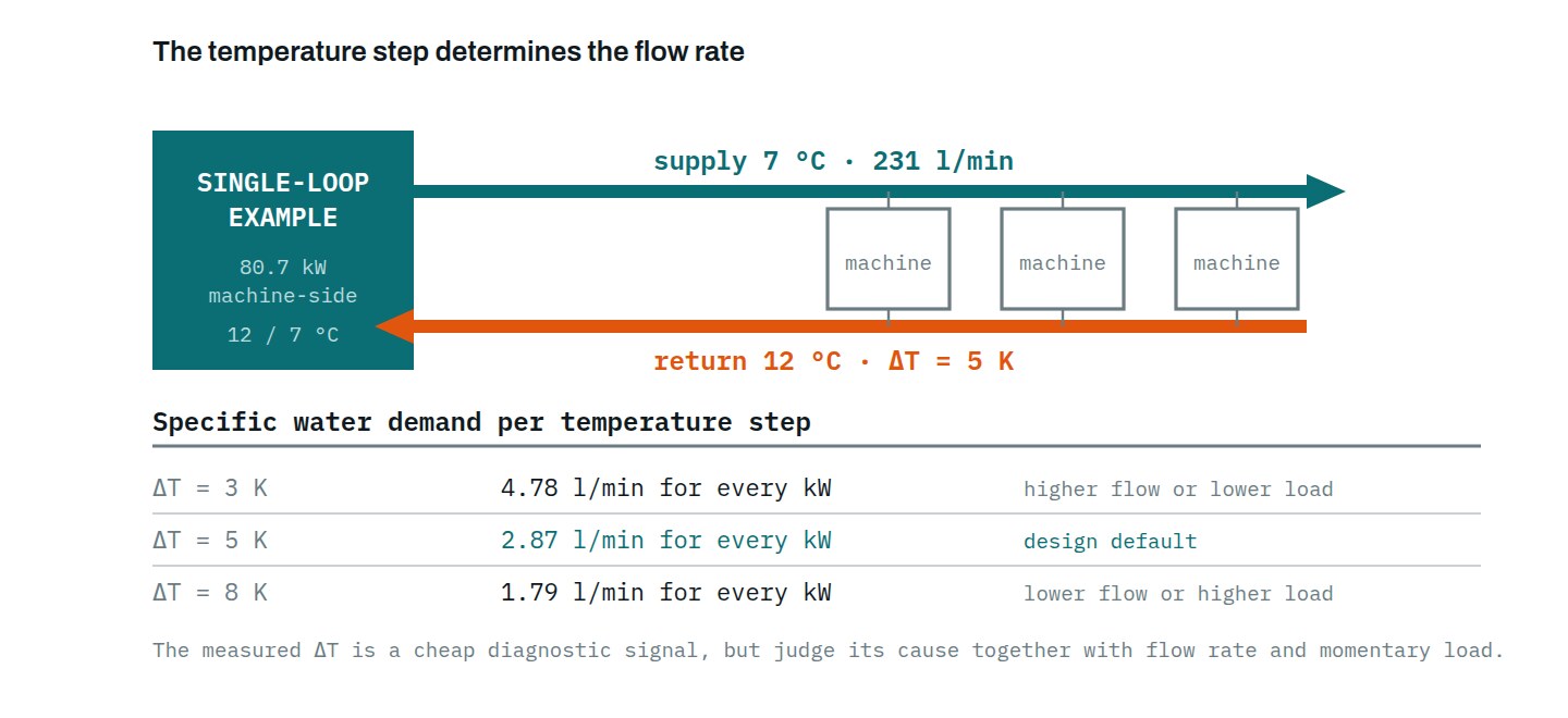
Cooling capacity on its own is worth nothing if the water does not reach the mould in sufficient quantity. The relationship:

V [l/min] = Q [kW] ÷ (ΔT [K] × 0.0698)

In practice this means that at a 5 K temperature step, every kilowatt needs roughly 2.9 l/min, i.e. 172 l/h of water. The 80.7 kW machine-side base load thus corresponds to about 231 l/min, i.e. 13.9 m³/h of flow. This is a flow rate calculated from the heat balance, and not automatically the final pump sizing figure: section 6 shows that the mould's turbulence requirement can force a larger one.

If the measured temperature step differs from the design value, that is a diagnostic signal, but by itself it does not tell you the cause. A lower ΔT can be caused by higher-than-design flow, a bypass left open, a momentarily lower heat load, or poor heat transfer in the mould. A higher ΔT can be caused by too little water, a clogged filter, or a momentarily higher load. Always evaluate the deviation together with the flow rate and the momentary load.

One practical sign worth remembering: if the temperature of the water flowing through the mould does not rise appreciably, that is suspicious. Possible causes include far more water passing through the loop than needed, or scale build-up on the inner wall of the cooling channels stopping the heat from reaching the water at all. The second case is the worse one, because it develops slowly and goes unnoticed for a long time. Even a relatively thin deposit can degrade heat transfer and reduce the free cross-section, because the deposit's thermal conductivity is a fraction of that of mould steel. The effect on cycle time, however, depends strongly on the mould's geometry and material and on the deposit's thickness and conductivity, so no universal multiplier is worth memorising.

What the system adds on its own

The heat load calculated at the machines is still not the whole picture. The cooling loop itself also generates and absorbs heat, and these items hurt most on the cold loop, where the base load is smallest.

• The circulation pump. Its shaft power ends up almost entirely in the water. A pump running at 3 kW shaft power is therefore 3 kW of extra load. (The electrical power on the motor's nameplate is higher; the difference leaves as motor loss to the environment.) On a 17 kW cold loop this is already close to twenty percent.
• Heat gain of the pipe network. Cold water in a warm hall warms continuously. The magnitude depends strongly on nominal diameter, pipe material, air movement and temperature difference, but on long, uninsulated distribution runs it can reach kilowatt scale.
• Condensation. The same dew-point problem as at the mould, only on the pipes. The latent heat of the condensing moisture is load, and the dripping water is a corrosion and safety risk.
• Buffer tank and fittings. Same logic as the pipes.

On the warm loop all of this works in reverse. A 25 °C hall practically does not warm 28 °C water, and insulation is far less critical there. This is another argument for separating the loops: not only the energy cost but also the insulation requirement concentrates on the cold loop.

These items are added in the second round of sizing, when the pump and the routing are known. It cannot be done earlier, because the pump size follows from the flow rate, which follows from the heat load.

06. The turbulence nobody talks about

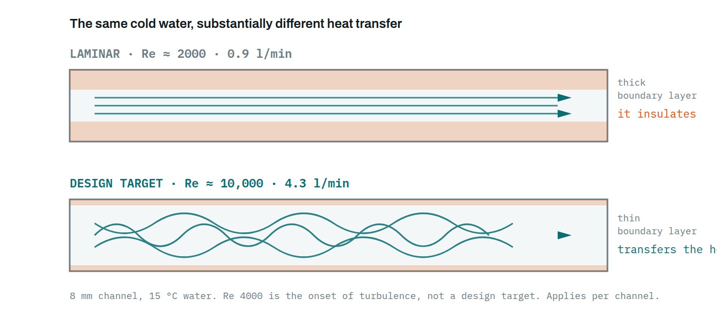
This is the point where most "the chiller is weak" complaints actually get solved. If the flow in the mould's cooling channel is laminar, a thick, motionless boundary layer forms along the wall, which behaves as thermal insulation. The water may be 7 degrees — the heat does not reach it.

The threshold is around a Reynolds number of 4000. In an 8 mm cooling channel this corresponds to roughly 1.7 l/min. But this is only the onset of turbulence, not the design target.

The literature recommends a higher target. The most frequently cited practical value is Re ≈ 10,000, on the grounds that above it the improvement in heat transfer flattens out, so pushing the flow further costs more in pumping than it delivers. For some geometries the measured optimum falls higher, so there is no universal target — but 4000 is definitely not it.

In numbers, for an 8 mm channel with 15 °C water:

Flow demand per channel (8 mm, 15 °C)

Reynolds number	l/min	What it means
4,000	1.7	onset of turbulence
6,000	2.6	turbulent, but not a design target
10,000	4.3	practical design target
20,000	8.6	measured optimum of some geometries

The values also depend on channel diameter and water temperature; recalculate for other diameters.

This is where it becomes clear why thinking about the mould loop purely in kilowatts is misleading. Our example machine's mould loop asks for 2.5 kW, which at a 5 K step would be barely 7 l/min. But on a mould with eight parallel cooling circuits, the Re ≈ 10,000 target needs 4.3 l/min per circuit — about 34 l/min in total. The actual temperature step will then not be 5 K but barely 1 K. (If the eight channel sections are connected in series in a single circuit, the same 4.3 l/min flows through all of them — so the difference between parallel and series layouts is an engineering-level one.)

This is not an error but the nature of the mould loop: the flow rate is dictated by the heat-transfer requirement, not by the heat quantity. The chiller sees the kilowatts; the mould asks for the litres per minute. The required flow is given by the larger of the two requirements, and the pump must then be selected from this flow and the whole system's pressure loss.

The same explains why 2.5 kW is not too little. It is not that the heat quantity is small for the mould — it is that there is no direct link between the heat quantity and the required water flow.

Where turbulence gets lost in practice

The flow needed for the target Reynolds number must be delivered against the whole loop's pressure loss. Long or narrow hoses, quick couplers, restrictions and long cooling channels all increase the system's resistance. If the pump's operating point shifts to a lower flow as a result, the Reynolds number can fall below target.

There is no universal permissible pressure-drop figure. The loop must be checked against the required flow and the available pump's characteristic curve.

One item almost never checked: the quick couplers. Overly long, overly narrow hoses with couplers on them are common in plants. The pressure loss of a valved quick coupler can be a multiple of a free-flow coupler of the same nominal size. Selection must therefore be based on the specific coupler's Δp–Q curve, not on nominal size.

In other words, the performance of a mould's cooling circuit is often limited neither by the chiller nor by the channel geometry, but by a few badly chosen couplers and one hose that is too long. It is the cheapest bottleneck to fix in the whole system.

And it is not only an energy issue: temperature-control faults carry significant scrap and quality risk, because unevenness in mould-wall temperature shows up directly in part warpage and surface.

07. What the catalogue figure does not tell you

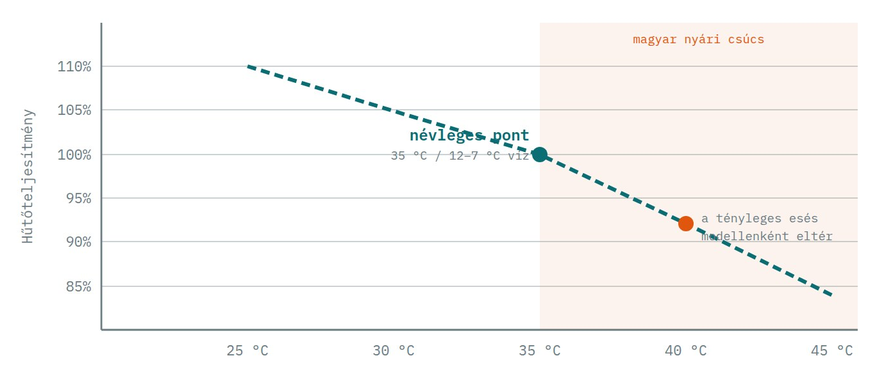
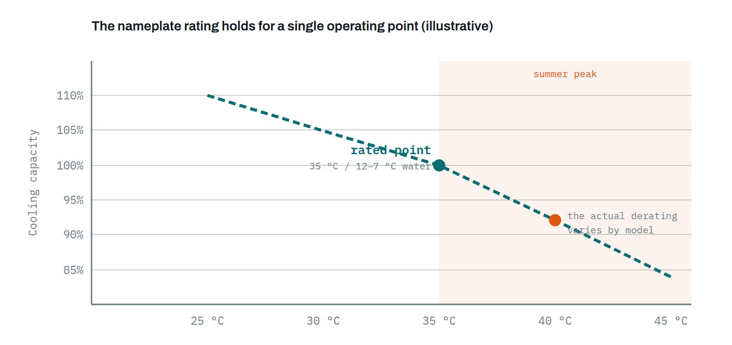
The cooling capacity on the datasheet is not a universal number but belongs to a specific measurement point: typically 12/7 °C water and 35 °C ambient. At higher ambient temperature the same air-cooled machine delivers less — precisely when it is needed most.

How much less cannot be generalised. It depends on the compressor, the condenser, the refrigerant, the supply water temperature and the specific model. At selection, therefore, always read the value belonging to your operating point from the manufacturer's capacity table. The iTech chillers' capacity tables state this per operating point.

Glycol: not a neutral ingredient

With an outdoor unit there is no way around frost protection, but glycol changes three things: it lowers the mixture's specific heat, raises its density, and substantially raises its viscosity. All three affect sizing, the last one especially the pump calculation. The required flow and the pump head must therefore be recalculated for the actual glycol concentration, using the glycol manufacturer's engineering data. If glycol enters the system later, the pump's original sizing becomes obsolete.

Refrigerant and regulation

The F-gas regulation, currently Regulation (EU) 2024/573, contains placing-on-market and servicing restrictions for certain refrigerants. This directly affects the conditions under which a given machine can be kept in operation over the investment's lifetime.

Ecodesign is a separate question: it sets minimum requirements not for the refrigerant but for the equipment's energy efficiency. The two sets of rules must be assessed separately in the investment decision.

08. The two-loop system: where the money is

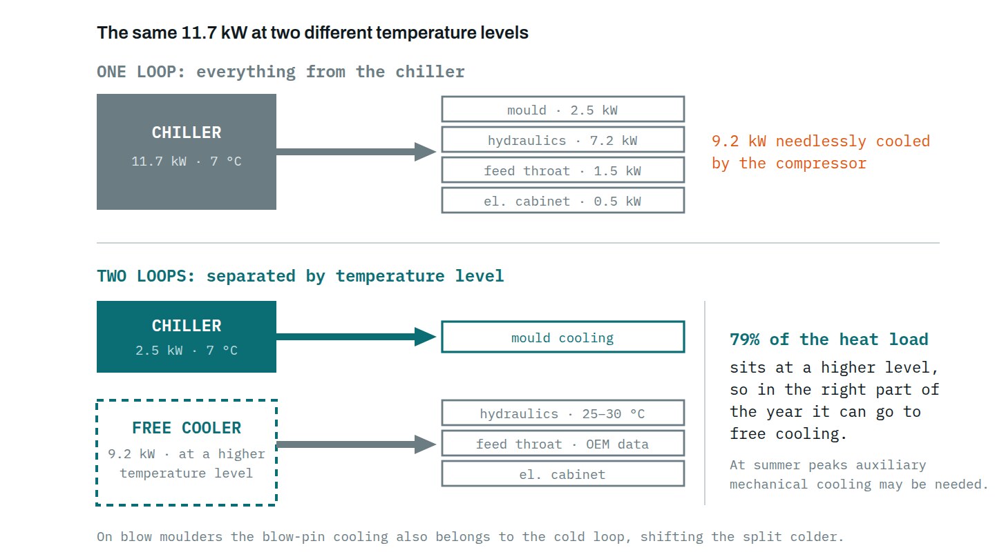
Looking through the four items, it turns out that only one of them genuinely requires cold water. Of the 11.7 kW per machine, the 2.5 kW of mould cooling asks for 7–15 °C. The hydraulic oil is fine with 25–30 °C, and the feed throat and the electrical cabinet cooler also run at a higher temperature level.

Per machine, then, 9.2 kW of the 11.7 kW — 79 percent of the heat load — occurs at a level that does not necessarily need a compressor. The lower the machine's specific throughput, the higher this share.

What a free cooler can do, and what it cannot

Precision matters here, because it is easy to overpromise. A dry free cooler can only remove meaningful heat when the outside air is sufficiently colder than the desired fluid temperature. The heat exchanger needs an approach temperature difference: a few degrees of gap is not yet enough driving force. If 25–30 °C water has to be held, a free cooler alone will not handle the warm loop on a 35 °C summer day.

The correct phrasing is therefore that a substantial share of the warm loop's heat load can be removed by free cooling in the right parts of the year. At high outside temperatures, supplementary mechanical cooling, a hybrid solution, or a higher water temperature approved by the machine manufacturer may be needed. Which is cheaper must be calculated with the site's climate data and the free cooler's sizing.

The two loops' calculated heat load

The machine-side base load of the cold loop's consumers is about 17 kW; that of the warm loop is about 64 kW.

These are still not the final cooling-equipment sizing figures. The loop's own loads from section 05 must be added: pump work, pipe-network heat gain, condensation. If, say, a pump with 3 kW shaft power works on the cold loop, the 17 kW is already around 20 kW before pipe heat gain. Only then comes equipment selection, per loop, based on the required water temperature and the design outdoor temperature.

This is the essence: do not select a machine for the 80.7 kW machine-side base load, but per loop, at each loop's own temperature level. The cold loop thus requires a substantially smaller chiller than the machine-side base load would suggest.

On blow moulding machines the split differs in that blow-pin cooling also belongs to the cold loop, since it cools the bottle neck directly and constrains the cycle time.

Separating the loops is the single largest one-off saving opportunity in a plastics plant's cooling — and exactly why it should be decided at the sizing stage. Retrofitting it is pipework reconstruction, not parameter tuning.

09. The sizing procedure, summarised

• Collect per machine the material, the hourly throughput, the drive-motor power and the drive technology.
• Calculate the melt heat with a material-specific Δh, preferably from the supplier's datasheet. Do not average for semi-crystalline materials.
• Add the hydraulic-oil load from manufacturer data or measurement, not from a template multiplier.
• Account for the feed throat temperature control, the electrical cabinet cooling and every other consumer on the same loop — on blow moulders the blow pin too. Request machine-manufacturer data for these.
• Do not count again the process heat the TCU removes from the mould.
• Mark for every item the temperature level at which it occurs. This decides what goes on the chiller.
• Only reduce for coincidence if you have time-series load data showing how many machines load the system simultaneously on a sustained basis. The productive-hours ratio alone is not enough. Without such data, do not reduce. The margin comes after this.
• Check the water side: is the flow sufficient, and is the flow turbulent per channel? On the mould loop the flow rate governs, not the kilowatts.
• Check the hoses and quick couplers too. One bad coupler can hurt a cooling circuit more than a bigger chiller can help.
• Check the hall's dew point at the design humidity, and choose the mould-loop water temperature accordingly. The chiller's outlet temperature and the mould loop's temperature are not the same thing.
• In the second round add the system's own items: pump power, pipe-network heat gain, condensation. With a hot-runner mould, the hot runner's heat input as well.
• Read the value for the design operating point from the manufacturer's capacity table, and calculate with the actual glycol concentration. Select equipment per loop, not for the total heat load in one go.

These twelve steps are half an hour's work once the data is at hand. And that is the half hour that decides how much you will pay for cooling over the next ten years.

Next in the series: Cooling-water treatment in production plants: why does the chiller nobody inspects break down? Water quality, scale build-up and measurement logging in practice.